software

HaasoscopePro Software

Python-based oscilloscope software for the HaasoscopePro hardware.

Quick Start

Installation

# Install dependencies from requirements file
pip install -r requirements.txt

# Or install manually
pip install numpy scipy pyqtgraph PyQt5 ftd2xx requests packaging

Note: requests and packaging are optional but recommended for automatic update checking.

Running with Hardware

# Run the application
python HaasoscopeProQt.py

The software will automatically detect connected HaasoscopePro boards via USB.

Running with Dummy Server (No Hardware Required)

For development and testing without physical hardware:

# Terminal 1 - Start dummy server
cd dummy_scope
python dummy_server.py --port 9999

# Terminal 2 - Run application with socket connection
python HaasoscopeProQt.py --socket localhost:9999

Command-Line Options:

# Single dummy board on custom port
python HaasoscopeProQt.py --socket localhost:9999

# Multiple dummy boards (multi-board simulation)
python HaasoscopeProQt.py --socket localhost:9998 --socket localhost:9999 --socket localhost:10000

# Remote dummy server
python HaasoscopeProQt.py --socket 192.168.1.100:9999

# Mix hardware and dummy boards (if hardware is detected, socket boards are added)
python HaasoscopeProQt.py --socket localhost:9999

# Limit maximum number of devices to connect (default: 100)
python HaasoscopeProQt.py --max-devices 4

# Testing mode (disables dynamic status bar updates for stable screenshots)
python HaasoscopeProQt.py --socket localhost:9999 --testing

# Combine options
python HaasoscopeProQt.py --max-devices 5 --socket localhost:9999 --testing

# Show help
python HaasoscopeProQt.py --help

Automatic Fallback: If no --socket is specified and no hardware is detected, the application automatically tries to connect to localhost:9998.

See dummy_scope/README.md for detailed dummy server documentation.

Editing the GUI

The Haasoscope Pro GUI can be edited using Qt Designer, on software/HaasoscopePro.ui or HaasoscopeProFFT.ui etc.

Keyboard Shortcuts

The GUI supports keyboard shortcuts for quick control adjustments:

Shortcut	Function
Arrow Keys
Left / Right	Decrease / Increase time scale (downsample)
Up / Down	Increase / Decrease offset
Shift + Arrow Keys
Shift+Up / Shift+Down	Increase / Decrease gain
Ctrl + Arrow Keys
Ctrl+Up / Ctrl+Down	Increase / Decrease trigger threshold
Ctrl+Left / Ctrl+Right	Decrease / Increase trigger position
Alt + Arrow Keys
Alt+Up / Alt+Down	Increase / Decrease trigger delta
Other Keys
Space	Toggle run/pause
R	Set rising edge trigger on current channel
F	Set falling edge trigger on current channel
T	Toggle two-channel mode for current board
C	Toggle between channel 0 and 1 (two-channel mode)
0 - 9	Select board 0-9

Tips:

• Arrow keys provide quick navigation without reaching for the mouse
• Modifier keys (Shift/Ctrl/Alt) access additional functions on the same arrow keys
• All shortcuts work when the main window has focus

Multi-Board Features

The Haasoscope Pro supports daisy-chaining multiple boards via LVDS for synchronized operation.

Automatic LVDS Delay Calibration

When multiple boards are connected, the system automatically calibrates and compensates for trigger signal propagation delays:

• Initial Setup: After PLL reset during startup, LVDS calibration runs automatically for the initial trigger board
• Switching Trigger Sources: When you set a different board to channel-based trigger (using R or F keys, or via UI), calibration runs automatically if no saved calibration exists
• Saved Calibrations: Each trigger source board has its own calibration set that is automatically restored when switching back

To use:

1. Start the application (PLL reset and LVDS calibration happen automatically)
2. Switch trigger sources as needed using keyboard shortcuts or UI - calibration is fully automatic!

Manual calibration is also available via Calibration → Board LVDS delays menu.

For detailed technical information, see EXTTRIG_ECHO_CALIBRATION.md.

Trigger Source Management

• Only one board can be self-triggering at a time (enforced automatically)
• When setting a board to channel-based trigger, all other boards are automatically set to external trigger mode
• Keyboard shortcuts make it easy to switch trigger boards:
  • 0-9: Select board
  • R: Set rising edge trigger on current board
  • F: Set falling edge trigger on current board

Board Synchronization

• Board Stabilizer: Corrects for trigger jitter on the self-triggering board
• Extra Trigger Stabilizer: Fine-grained per-frame stabilization applied across all boards
• LVDS Compensation: Firmware (coarse) + software (fine) dual-layer delay compensation for sample-level precision

Code Architecture

This diagram shows the software architecture with all major components, data flows, and relationships. Use mermaid.live to convert it to diagram.png.

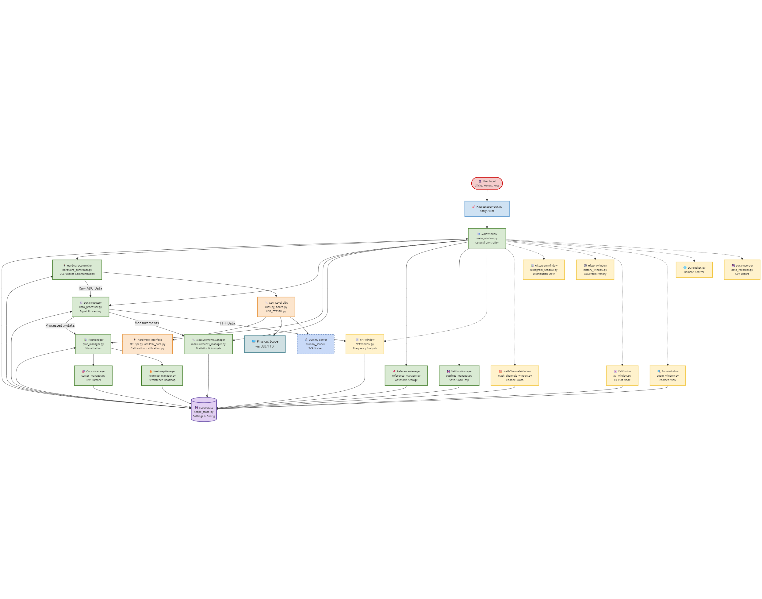
graph TD
    %% --- Styling Definitions ---
    classDef core fill:#d9ead3,stroke:#38761d,stroke-width:2px,font-size:12px;
    classDef startup fill:#cfe2f3,stroke:#3d85c6,stroke-width:2px,font-size:12px;
    classDef hardware fill:#fce5cd,stroke:#e69138,stroke-width:2px,font-size:12px;
    classDef helpers fill:#fff2cc,stroke:#f1c232,stroke-width:2px,font-size:12px;
    classDef datastore fill:#e2d0f3,stroke:#674ea7,stroke-width:2px,font-size:12px;
    classDef user fill:#f4cccc,stroke:#cc0000,stroke-width:2px,font-size:12px;
    classDef device fill:#d0e0e3,stroke:#45818e,stroke-width:2px,font-size:14px;
    classDef testing fill:#c9daf8,stroke:#1c4587,stroke-width:2px,font-size:12px,stroke-dasharray:5;

    %% --- Entry Point ---
    User(["👤 User Input<br>Clicks, Menus, Keys"]) -.-> A
    A["🚀 HaasoscopeProQt.py<br><i>Entry Point</i>"] --> B

    %% --- Main Controller ---
    B["🎛️ MainWindow<br>main_window.py<br><i>Central Controller</i>"]

    %% --- Central State ---
    C[("💾 ScopeState<br>scope_state.py<br>Settings & Config")]

    B <--> C

    %% --- Core Processing Components ---
    B --> D["🔌 HardwareController<br>hardware_controller.py<br>USB/Socket Communication"]
    B --> E["⚙️ DataProcessor<br>data_processor.py<br>Signal Processing"]
    B --> F["📊 PlotManager<br>plot_manager.py<br>Visualization"]

    D <--> C
    E <--> C
    F <--> C

    %% --- Owned Managers ---
    B --> M1["📏 MeasurementsManager<br>measurements_manager.py<br>Statistics & Analysis"]
    B --> M2["📌 ReferenceManager<br>reference_manager.py<br>Waveform Storage"]
    B --> M3["💾 SettingsManager<br>settings_manager.py<br>Save/Load .hsp"]

    M1 --> C
    M2 --> C
    M3 --> C

    %% --- Plot Manager Owned Components ---
    F --> P1["🎯 CursorManager<br>cursor_manager.py<br>H/V Cursors"]
    F --> P2["🔥 HeatmapManager<br>heatmap_manager.py<br>Persistence Heatmap"]

    P1 --> C
    P2 --> C

    %% --- Popup Windows ---
    B -.-> W1["📈 FFTWindow<br>FFTWindow.py<br>Frequency Analysis"]
    B -.-> W2["🧮 MathChannelsWindow<br>math_channels_window.py<br>Channel Math"]
    B -.-> W3["📊 HistogramWindow<br>histogram_window.py<br>Distribution View"]
    B -.-> W4["🕐 HistoryWindow<br>history_window.py<br>Waveform History"]
    B -.-> W5["📉 XYWindow<br>xy_window.py<br>XY Plot Mode"]
    B -.-> W6["🔍 ZoomWindow<br>zoom_window.py<br>Zoomed View"]

    W1 --> C
    W2 --> C
    W5 --> C
    W6 --> C

    %% --- Data Flow ---
    D -- "Raw ADC Data" --> E
    E -- "Processed xydata" --> F
    E -- "Measurements" --> M1
    E -- "FFT Data" --> W1

    %% --- Hardware Layer ---
    D --> H1["🔧 Low-Level Libs<br>usbs.py, board.py<br>USB_FT232H.py"]
    H1 --> H2["🔌 Hardware Interface<br>SPI: spi.py, adf435x_core.py<br>Calibration: calibration.py"]

    H1 --> DEV1["🖥️ Physical Scope<br>via USB/FTDI"]
    H1 --> DEV2["🔬 Dummy Server<br>dummy_scope/<br>TCP Socket"]

    %% --- Additional Services ---
    B -.-> S1["🌐 SCPIsocket.py<br>Remote Control"]
    B -.-> S2["💾 DataRecorder<br>data_recorder.py<br>CSV Export"]

    %% --- Style Applications ---
    class A startup
    class B core
    class C datastore
    class D,E,F core
    class M1,M2,M3,P1,P2 core
    class W1,W2,W3,W4,W5,W6 helpers
    class H1,H2 hardware
    class DEV1 device
    class DEV2 testing
    class S1,S2 helpers
    class User user

Loading

Key Modules

Core Components

main_window.py - Main application controller

• Handles all UI events (clicks, menus, keyboard shortcuts)
• Orchestrates data flow between hardware, processing, and display
• Manages all component lifecycles
• Implements per-channel/per-board setting synchronization

scope_state.py - Central state storage

• Single source of truth for all oscilloscope settings
• Per-channel settings: gain, offset, AC/DC, impedance, resamp, peak detect, persistence
• Per-board settings: trigger settings, channel modes, pulse stabilizer
• Global settings: timebase, downsample, display options

hardware_controller.py - Hardware abstraction layer

• Manages communication with oscilloscope boards
• Sends low-level commands (SPI, trigger, gain/offset)
• Retrieves waveform data packets
• Supports both USB (FTDI) and socket (dummy server) connections

data_processor.py - Signal processing

• Processes raw ADC data into calibrated waveforms
• Calculates FFT spectra
• Computes measurements (Vpp, RMS, frequency, duty cycle, rise time)
• Applies calibration corrections

plot_manager.py - Display and visualization

• Renders waveforms using PyQtGraph
• Applies FIR frequency response correction
• Applies Savitzky-Golay polynomial filtering
• Manages per-channel peak lines, persistence, references
• Handles XY plot mode
• Cursor and measurement overlays
• Real-time plot updates

frequency_calibration.py - FIR calibration system

• Automatic frequency response correction using square wave calibration
• Support for all modes: normal (3.2 GHz), two-channel (1.6 GHz), oversampling, and interleaved (6.4 GHz)
• Measures duty cycle, frequency, and DC offset from input signal
• Adaptive tap count (32/64/128) based on sample rate
• Save/load calibration files (.fir format)
• See FIR_CALIBRATION_README.md for details

Supporting Components

FFTWindow.py - FFT spectrum analyzer window

• Real-time frequency domain display
• Per-channel FFT enable/disable
• Peak detection and analysis

math_channels_window.py - Math channel operations

• Channel arithmetic (add, subtract, multiply, divide)
• Mathematical functions (differentiate, integrate, smooth, envelope, abs, square, sqrt, log, exp)
• Digital filters (low-pass, high-pass, band-pass, band-stop) with Butterworth and Chebyshev designs
• Time shift with sub-sample interpolation (0.001 Hz to 10 GHz range)
• AC coupling and min/max tracking
• Custom expression evaluation

Implementation Note: Math channels are calculated from non-resampled source data (before doresamp is applied) to ensure correct FFT frequency ranges and optimal filter performance. Results are then resampled for display to match the source channel's resampling setting. This ensures that:

• FFT analysis shows the true Nyquist frequency of the source data
• Digital filters operate at the actual hardware sample rate
• Min/Max tracking automatically handles array size changes when doresamp is modified

xy_window.py - XY Plot window

• Displays Lissajous figures and parametric plots
• Plots one channel against another (X vs Y)
• Supports both physical and math channels
• Channel selection via dropdown menus
• Useful for I-V curves, phase relationships, and parametric analysis
• Accessed via View menu → XY Plot

zoom_window.py - Zoom window

• Synchronized zoomed view of the main plot
• Shows all active channels, math channels, and references
• Displays trigger lines, cursors, peak detect, and persistence
• Region of Interest (ROI) selection on main plot
• Secondary Y-axis for voltage display
• Non-interactive view (pan/zoom controlled by ROI on main plot)
• Cross-window mouse pointer (20-pixel crosshair visible only within ROI)
• Accessed via View menu → Zoom Window

histogram_window.py - Histogram display

• Statistical distribution visualization
• Waveform amplitude analysis
• Histogram binning and counting

history_window.py - Waveform history viewer

• Stores previous waveform captures
• Allows review of historical data
• Sequential playback of captured waveforms

measurements_manager.py - Measurements display

• Automated measurement calculations
• Statistics table display
• Rise time and edge analysis

reference_manager.py - Reference waveform management

• Store and recall waveforms
• Per-channel reference display
• Waveform comparison

cursor_manager.py - Cursor controls

• Horizontal/vertical cursors
• Delta measurements
• Snap to waveform
• Rise time fit visualization

heatmap_manager.py - Persistence heatmap visualization

• Density-based visualization of persist lines
• Adaptive resolution based on zoom level (1000x200 bins)
• Gaussian smoothing for professional appearance
• Color-coded density (blue-to-red gradient)
• Automatic regeneration on pan/zoom/gain changes

settings_manager.py - Settings persistence

• Save/load configuration files (.hsp)
• Backward compatibility handling
• Per-channel/board settings migration

data_recorder.py - Data logging

• CSV export
• Event capture
• Waveform recording

Hardware Communication

usbs.py - USB device management

• FTDI device discovery and initialization
• Socket device connections (for dummy server)
• Multi-board detection and ordering

board.py - Low-level board commands

• SPI communication
• PLL configuration
• Fan control, temperature reading
• Clock distribution for multi-board setups

USB_FT232H.py - FTDI wrapper

• Synchronous FIFO mode (FT232H)
• High-speed USB data transfer

dummy_scope/ - Testing framework

• TCP socket-based oscilloscope simulator
• Configurable waveform generation (sine, square, pulse)
• Full protocol implementation
• Multi-board simulation support

Utility Modules

calibration.py - Calibration data management

SCPIsocket.py - SCPI remote control interface

spi.py - SPI communication helpers

utils.py - Common utility functions

Data Flow

1. Acquisition: hardware_controller.get_event() retrieves raw ADC data from board
2. Processing: data_processor.process_board_data() converts to calibrated waveforms
3. Display: plot_manager.update_plots() renders waveforms on screen
4. Analysis: data_processor.calculate_measurements() computes measurements
5. FFT: Optional FFT analysis in FFTWindow

Configuration Files

Settings are saved in .hsp files (JSON format):

• Window geometry and UI state
• Per-channel settings (gain, offset, colors, persistence, resamp)
• Per-board settings (trigger, modes, pulse stabilizer)
• Display preferences (grid, cursors, markers)
• Math channel definitions
• Reference waveforms
• FIR and polynomial filtering enable states

FIR calibration data is saved separately in .fir files (JSON format):

• FIR coefficients for all modes (normal, two-channel, oversampling, interleaved)
• Sample rates and frequency response data
• Calibration metadata (timestamp, parameters)

Backward Compatibility: The settings manager automatically converts old single-value settings (resamp, peak detect, pulse stabilizer) to per-channel/board arrays when loading legacy files.

Development

Building Standalone Executables

# Windows
windowspyinstaller.bat

# macOS
./macpyinstaller.sh

# Linux
./linuxpyinstaller.sh

Executables are created in dist/ directory.

Adding New Per-Channel Settings

1. Add array to scope_state.py:

   self.my_setting = [default_value] * (num_boards * num_chan_per_board)

2. Update GUI in main_window.py select_channel():

   self.ui.mySettingBox.setValue(s.my_setting[s.activexychannel])

3. Add change handler:

   def my_setting_changed(self, value):
       self.state.my_setting[self.state.activexychannel] = value

4. Update settings_manager.py for save/load with backward compatibility

Adding New Per-Board Settings

Same pattern as per-channel, but use s.activeboard instead of s.activexychannel.

Code Style

• Follow existing naming conventions (snake_case for functions, CamelCase for classes)
• Document complex algorithms with inline comments
• Use type hints where helpful
• Keep UI logic in main_window.py, processing in separate modules

Troubleshooting

ImportError: No module named 'PyQt5'

pip3 install PyQt5 pyqtgraph

FTDI device not found

• Install FTDI D2XX drivers (see main README)
• Check USB connection (5V 2A minimum)
• Verify device appears in system device manager

Slow performance

• Reduce persistence time
• Disable peak detect when not needed
• Close FFT window when not in use

Dependencies

All dependencies are listed in requirements.txt and can be installed with:

pip install -r requirements.txt

Core Dependencies

• Python 3.7+ (3.8+ recommended)
• PyQt5 - GUI framework
• pyqtgraph - Fast plotting library
• numpy - Numerical computing
• scipy - Signal processing (FFT, filtering, interpolation)
• ftd2xx - FTDI driver wrapper for hardware communication

Optional Dependencies

• requests - For automatic update checking (gracefully degrades if not installed)
• packaging - For version comparison in update checker

License

Same as parent HaasoscopePro project.

See Also

• Main Project README
• Dummy Server Documentation
• Firmware Documentation
• Hardware Schematics
• HaasoscopePro on Hackaday.io